Building the Active Sweet Receptor from a Cloud of Density
A walkthrough of how to build an atomic model from a cryo-EM density map
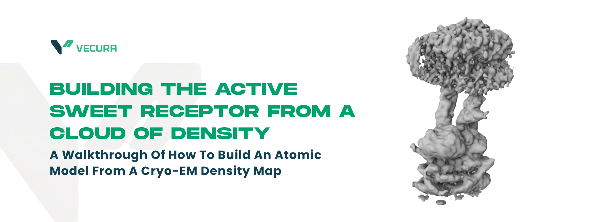
A walkthrough of how to build an atomic model from a cryo-EM density map
Every time you taste something sweet, a single protein on your tongue is doing the work: the human sweet taste receptor, a partnership of two proteins called TAS1R2 and TAS1R3. Sugar, sucralose, stevia, aspartame — they all register as "sweet" because they switch this one receptor on. To study how that switch works, you need a three-dimensional atomic picture of the receptor in its switched-on state.
This post is a practical walkthrough of how to get that picture — how to turn a fuzzy experimental density map into a clean, chemically valid atomic model. The sweet receptor makes an unusually good teaching case, because the activated state exists only as a density map, with no finished model to download. So every part of the model has to be built, and each step exposes a general technique: tracing a chain into density, assigning sequence, grafting domains from a second structure, editing a ligand, repairing gaps, and validating the result against the map. It's a story about how much of modern structural biology is careful assembly rather than direct observation.
Try this workflow on Vecura: Open the workflow
The receptor, and why "active" is the hard part
The sweet receptor belongs to a family called Class C GPCRs (G-protein-coupled receptors). Think of each half of the receptor as having two main pieces connected by a short tether:
-
A large Venus flytrap domain (VFT) sticking out of the cell, where sugars and most sweeteners actually bind. It's named for the way it closes around a ligand like the carnivorous plant snapping shut.
-
A seven-helix transmembrane domain (7TM) buried in the cell membrane, which passes the signal to the inside of the cell.
When a sweetener lands in the flytrap and it closes, that motion travels down through a small cysteine-rich domain (CRD) linker and rearranges the 7TM helices. That rearrangement is the "on" switch that the cell reads out.
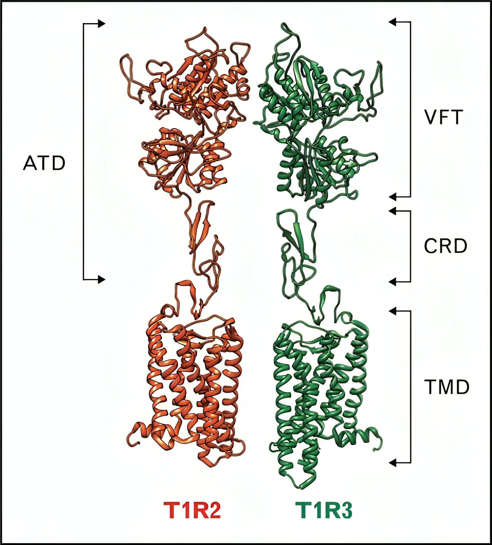
Figure 1. TAS1R2/TAS1R3 heterodimer showing the VFT, CRD, and 7TM domains.
The 7TM is worth dwelling on, because it's where the most interesting pharmacology happens. The flytrap is the orthosteric site — where the sweetener itself binds. But buried inside the seven-helix bundle of the TAS1R3 subunit is a second, separate pocket: the allosteric site. Molecules that bind there don't taste sweet on their own and don't compete with the sugar; instead they tune the receptor's response to whatever is in the flytrap. Two flavors matter:
-
Positive allosteric modulators (PAMs) — enhancers. They stabilize the active shape, so a given amount of sugar produces a stronger signal. This is the holy grail for the food industry: a PAM could let a product taste as sweet with a fraction of the sugar, because it amplifies the sweetness you already have rather than adding calories of its own.
-
Negative allosteric modulators (NAMs) — inhibitors. Lactisole is the textbook example: it binds this 7TM pocket and shuts sweetness off, which is why it reads as a sweetness suppressor. Its potency hinges on a couple of specific pocket residues (a histidine and a glutamine deep in the bundle), which is exactly the kind of detail an atomic model has to get right.
Here's the crux for this walkthrough. That allosteric pocket is lined by the very helices — especially TM5 and TM6 — that move when the receptor switches on. So the shape of the pocket, and therefore which modulators can bind and how tightly, is different in the active state than in the resting state. To study enhancers or inhibitors of sweetness with any confidence, you need an atomic model of the 7TM in its active shape, not its resting shape. That is the model this walkthrough builds.
Here's the catch. When we surveyed the available experimental structures, the best full-length human structure of the receptor — a cryo-EM structure known by its database code 9UTB, solved with sucralose bound — had its flytrap closed but its 7TM still in the inactive shape. The sweetener was sitting in the pocket, but the transmembrane switch hadn't flipped in the frozen sample. We confirmed this by comparing it to the apo (ligand-free) structure: the two 7TMs were nearly identical. So the one structure that was human and full-length couldn't tell us what the active 7TM looks like.
The active conformation existed in only one place: a cryo-EM density map called EMD-70734.
What a density map is (and isn't)
Cryo-electron microscopy doesn't hand you an atomic model. It gives you a map — a three-dimensional cloud showing where the electrons in a flash-frozen sample were dense. Where the protein is, the cloud is thick; where there's empty solvent, it's thin. A researcher's job is to thread a chain of atoms through that cloud so the atoms sit where the density is.
How easy that is depends on resolution, measured in ångströms (Å, ten-billionths of a meter). At 2 Å you can see individual atoms. EMD-70734 was solved at 4.28 Å — good enough to trace the path of the backbone and see the sausage-like shapes of helices, but not good enough to read off which amino acid is which or to place side chains reliably. It's like a satellite photo where you can make out streets and buildings but not house numbers.
Crucially, this map captured the receptor in what its authors called the "loose" state — the activated conformation we needed, with sucralose bound. No one had deposited a finished atomic model for it — we confirmed this against the EMDB, whose fitted-model listing for EMD-70734 is empty. So we had to build one.
Step 1 — Trace the helices from the cloud
Before building anything, we first sharpened the map itself. At 4.28 Å the raw density is smeared, so we ran it through CryoSAMU, a deep-learning tool built specifically for intermediate-resolution maps. It uses a neural network (a "structure-aware multimodal U-Net") that pairs the density with structural expectations learned by a protein language model, and outputs a cleaner, more interpretable map. Think of it as computationally de-blurring the satellite photo before trying to read it: the helices come out crisper and easier to trace.
On that enhanced map we then ran CryoAtom (CryoAtom2), an automated model-building program that goes from density straight to an atomic structure. Under the hood it predicts where the backbone atoms sit, assembles them into an all-atom chain, and can even identify the sequence by searching a proteome database against the density — with a final clean-up step adapted from an earlier tool, ModelAngelo.
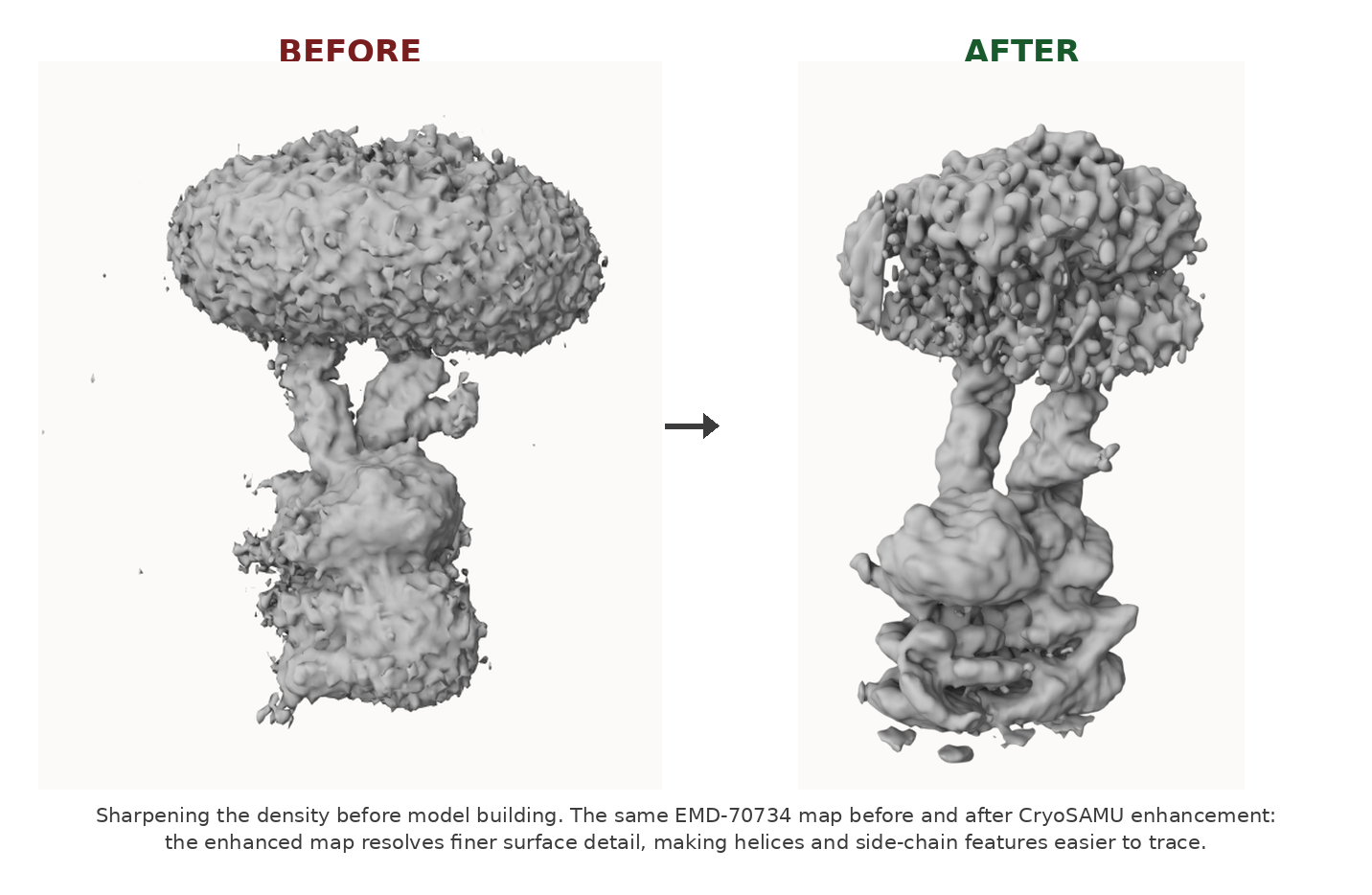
Figure 2. Sharpening the density before model building. The same EMD-70734 map before and after CryoSAMU enhancement. The enhanced map resolves finer surface detail, making helices and side-chain features easier to trace.
The raw result was still messy, in a telling way: it contained about 27,000 atoms across 900-plus little chain fragments, roughly twice as many residues as the receptor actually has. Even after enhancement, at this resolution the algorithm can't cleanly tell protein from noise, so it over-builds, fitting bits of chain into blobs that aren't really there.
Cleaning this up meant deciding, fragment by fragment, which pieces belonged to TAS1R2, which to TAS1R3, and which were noise. We did this by aligning each fragment against known reference structures and letting the best geometric fit vote. What survived was the part that mattered: fourteen transmembrane helices — seven per subunit — with a reliable backbone trace. Individual helices matched the reference geometry to within about 2.6–3.9 Å, all better than the map's own resolution, which is the sign that the backbone path is trustworthy even though the fine detail isn't.
At this stage we had helix positions but not helix identities — a shape, not a sequence.
Step 2 — Check that this is genuinely the "on" state
Before investing more work, we had to be sure the loose-state 7TM was truly a different conformation from the inactive structures, and not just experimental scatter. So we compared it against the inactive compact and apo structures along the metrics that define Class C GPCR activation.
The signatures all lined up. The two subunits' TM6 helices — the interface that opens up to let the G-protein dock inside the cell — had separated by about 2.6 Å, exactly the kind of opening activation is supposed to produce. TM5, the helix that lines the drug pocket, had swung dramatically (over 8 Å in one subunit), reshaping the pocket. And the allosteric pocket itself had contracted by roughly 15%, becoming narrower and deeper. Nine independent structural criteria for "active vs. inactive" all pointed the same way. This wasn't noise; it was the switch caught mid-flip.
That mattered for a practical reason too: it meant a docking pocket built from this map would actually differ from the inactive pocket, so it could tell PAMs (which prefer the active shape) apart from inhibitors (which prefer the inactive one).
Step 3 — Give the helices the right identity, and make them human
The map's helices came with the wrong labels in two senses. First, side chains were essentially unassigned. Second, the closest inactive 7TM reference available for one subunit came from a mouse version of TAS1R3, and mouse and human sweet receptors differ at dozens of positions — including several that line the very pocket we care about.
So we rebuilt the sequence. Using the human TAS1R3 sequence as the template, we applied 58 mouse-to-human substitutions, six of which sit directly in the allosteric pocket (for example, swapping a mouse alanine for the human serine at the key pocket position, and a histidine for an arginine). Missing atoms and hydrogens were added back computationally. We then nudged the side chains to better match the experimental density where the map could constrain them, and did a gentle energy minimization to relieve strain — while holding the backbone almost perfectly still (it moved less than half an ångström on average). The backbone came from the experiment; only the chemistry got corrected.
The result was active_7tm_human.pdb: a genuinely human, genuinely active 7TM domain. But it was only half a receptor — floating helices with no flytrap on top.
Step 4 — Graft the active 7TM onto a full-length body
This is where the two data sources come together. The full-length structure 9UTB had exactly what our 7TM model lacked — a well-resolved, already-human VFT and CRD with sucralose bound in the flytrap. Its only flaw was the inactive 7TM. Our EMD-70734 model was the reverse: a good active 7TM with no body.
The plan almost writes itself: keep the flytrap and linker from 9UTB, snap off its inactive 7TM, and graft our active 7TM in its place. The two came from different experiments in different coordinate frames — tens of ångströms apart in space — so we aligned them using the short stretch of backbone right at the CRD-to-7TM junction, the natural seam where the two pieces meet.
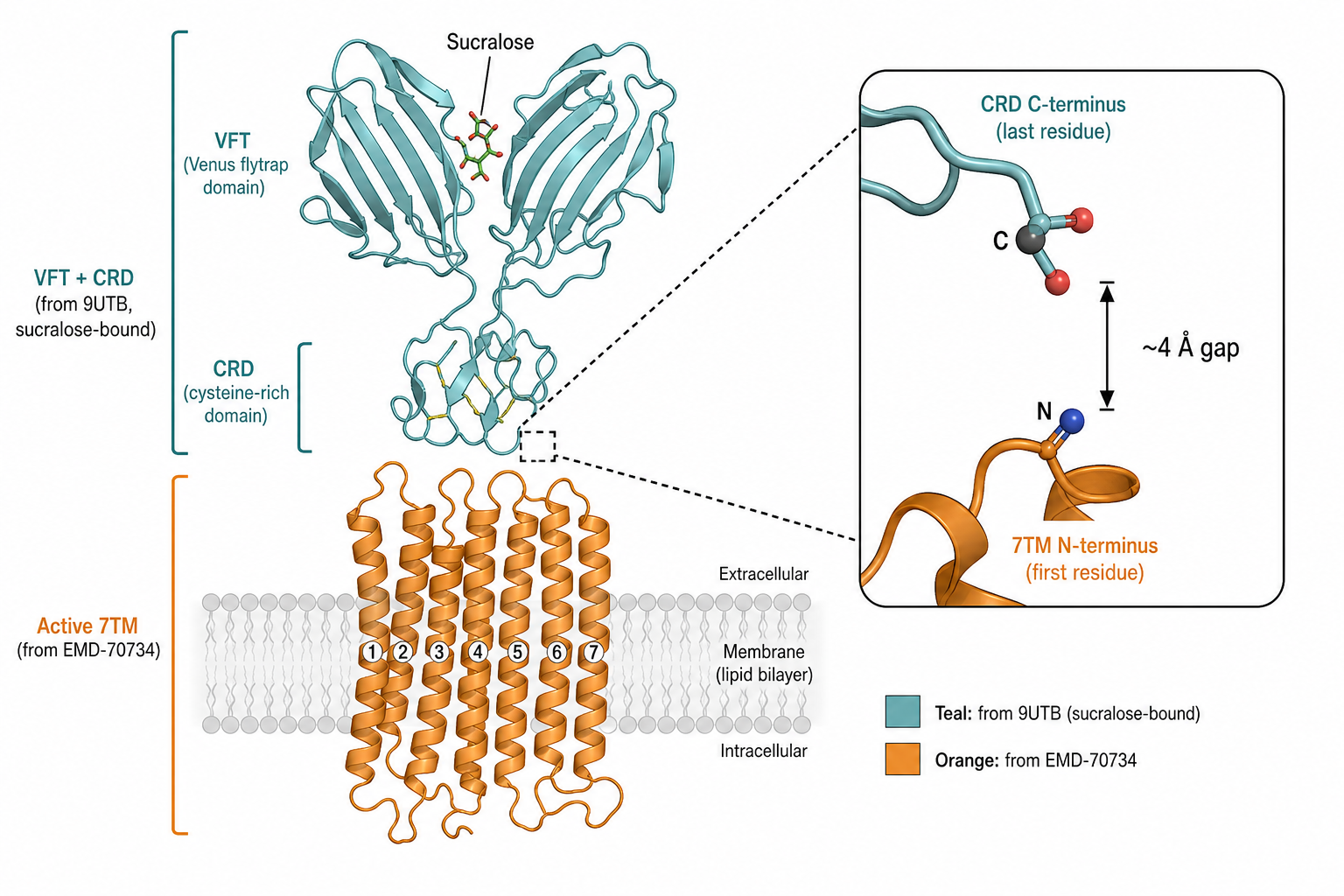
Figure 3. Building a composite. The well-resolved flytrap and linker from 9UTB are joined to the active 7TM from the density map at the CRD–7TM junction (inset).
The seam didn't close perfectly on the first try, and it wasn't supposed to. After alignment the gap across the junction was about 4.1–4.4 Å, versus the 3.8 Å of a normal chemical bond — a small overshoot that reflects the real rotation the 7TM undergoes during activation (the two pieces are, after all, in different functional states). That last fraction of an ångström is exactly what energy minimization is for.
Step 5 — Swap the ligand: sucralose to sucrose
Both experimental sources used sucralose (the artificial sweetener in Splenda) rather than table sugar, because sucralose gives sharper density. But we wanted a sucrose-bound model as our reference. Chemically the two molecules are almost identical: sucralose is sucrose with three chlorine atoms swapped in for three hydroxyl (–OH) groups. So we did the reverse edit — removed the three chlorines and rebuilt the hydroxyls in their place, adjusting the bond lengths to match. Three atoms changed per site; everything else stayed put.
Step 6 — Make it one continuous, physically valid molecule
A subtle problem nearly derailed the assembly. The stitched-together model had internal breaks — places where the chain stopped and restarted — partly from the grafting and partly from two loops (12 and 15 residues long) that the original experiment never resolved. Molecular simulation software reads a protein as continuous chains, and these breaks made it throw errors: it couldn't recognize residues sitting at unexpected chain ends, and it invented spurious bonds across gaps.
The fix was structural bookkeeping done carefully: merge the fragments into two clean chains (one per subunit) and fill the two missing loops using the known human sequence. After adding hydrogens at physiological pH, the model came to about 25,000 atoms and — importantly — loaded into the simulation software cleanly, with no special override flags. Continuous chains, valid chemistry.
(One honest caveat: the two rebuilt loops float out into space, far from the protein body, because there was no density to anchor them. Their internal geometry is fine, and they sit more than 100 Å from the drug pocket, so they don't affect the docking work — but they're a reminder that "filled in" is not the same as "observed.")
Step 7 — Relax the model, without letting it fall apart
The final shaping step is energy minimization: let the software adjust atomic positions to relieve clashes and settle bonds into comfortable lengths. Done naively, this would let the whole structure drift away from the experimental data. So we minimized with restraints — think of them as springs of different stiffness holding different regions in place.
The well-determined flytrap and linker were held almost rigidly. The active 7TM was held moderately, allowing local relaxation while preserving its activated shape. The junction seam and the rebuilt loops were left soft, free to settle. (Getting the restraint strengths to apply region-by-region actually required fixing a bug in our own script — a global stiffness value was quietly overriding the per-region ones, freezing everything equally. Worth mentioning because these mundane software details are where real models silently go wrong.)
After minimization the seam had closed to a proper chemical bond (3.86–3.88 Å across the junction, a textbook 1.34 Å peptide bond), there were zero atomic clashes, all 17 disulfide bonds were intact, and the pocket residues sat where they should. When we re-added sucrose, a couple of iterations of nudging resolved the last few clashes with the ligand barely moving.
The output, model_a_sucrose_minimized.pdb, was the deliverable: a full-length, human, active-state, sucrose-bound sweet receptor, about 25,000 atoms, chemically valid and simulation-ready.
The finished structure
At this point the workflow is complete. The deliverable is model_a_sucrose_minimized.pdb: a full-length, human, active-state, sucrose-bound sweet receptor — roughly 25,000 atoms, two continuous chains, ligand in the flytrap, chemically valid and ready to load into any downstream tool. It's a single self-consistent file assembled from pieces that no single database entry contained.
But before trusting it, there's one more step the build itself doesn't guarantee: checking that the finished model actually matches the map it was supposed to come from.
How well does the model actually fit the data?
A model can be clash-free and chemically valid and still not match the density it was supposed to come from. So we went back and tested the finished structure directly against the EMD-70734 map — the validation step the original build had skipped.
The good news first. The active 7TM does sit in the map, in the right place. Around 80% of its atoms fall on above-average density, and when we compared its fit to twelve randomly displaced copies of the same model, the real placement scored far above that random background and couldn't be improved by nudging it a few ångströms in any direction. In other words, it is genuinely registered in the density, not floating in noise, and not obviously mis-positioned.
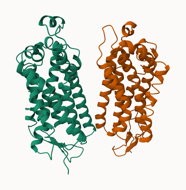
Figure 4. The backbone tracks the density well, but side chains are only loosely constrained, the visual counterpart of a ~0.40 correlation at 4.28 Å.
The honest news is that the quality of that fit is only modest. The standard measure — a map–model cross-correlation — came out around 0.40 (on a scale where a well-refined structure at this resolution typically reaches 0.6–0.75). That number tells a consistent story: the backbone was traced into the density and the side chains were rebuilt from the human sequence, but the model was never real-space refined — the step where you let the atoms settle into the map itself. The helices are in the right neighborhood; the finer pocket geometry is not yet pinned down by the experiment.
This sets the ceiling on what the model can be used for. Fine details — the exact placement of side chains lining a pocket, differences on the order of a few ångströms — sit below what a 0.40-correlation fit can support. Two other checks reinforced the caution: the isolated 7TM has 22 cysteines but none are modeled as forming disulfide bonds, so the extracellular loops are under-constrained; and the two computationally rebuilt loops, while internally sensible, still hang away from the protein body because no density anchors them.
The takeaway isn't that the model is wrong — it's that it's provisional. It's a well-placed, internally clean interpretation of a low-resolution cloud. The obvious next step, and the one that closes the loop on this workflow, is real-space refinement: letting the atoms settle into the map itself (with a tool like phenix.real_space_refine or ISOLDE) to push that correlation up before the fine geometry is trusted.
A second route: building a glucose-bound state with molecular dynamics
The model above answers "what does the active, sucrose-bound receptor look like?" A natural follow-on question is "what about a different sugar — say glucose?" You might think you could just swap glucose for sucrose the way we swapped sucralose earlier. But glucose is half the size of sucrose and grips the flytrap differently, so the pocket has to relax around it. That's a job for a different technique: molecular dynamics (MD), where you place the receptor in a simulated environment and let the atoms move under physical forces for a stretch of time.
So the second model starts from the first: dock glucose into the flytrap of the sucrose-built model, then run a 100-nanosecond simulation and let the receptor settle around the new ligand. That raises a problem unique to MD — the simulation doesn't produce one structure, it produces a movie of nearly two thousand snapshots. Which frame is the model? Picking one is its own small discipline.
Choosing a frame, on the evidence
Rather than eyeball it, each candidate frame was scored on three things that actually matter for a usable model, then combined into a single weighted number:
-
Does the glucose stay put? A frame where the sugar has drifted out of the binding site is useless, no matter how nice the protein looks (25% of the score).
-
Is the 7TM still in the active shape? Measured against the sucrose model as the active-state reference — helix positions, the hallmark TM6 opening, the pocket backbone (40%, the largest weight, because the whole point is an active model).
-
Is the drug pocket well-formed? A real, open cavity with no ions clogging it (35%).
The 10-nanosecond frame won decisively — top of all three categories, with a composite score of 0.91 versus 0.63 for the runner-up. It kept glucose in the pocket touching all five key sweetener residues, stayed closest to the active reference (helix deviations ~1.3 Å), and had the most reference-like pocket shape.
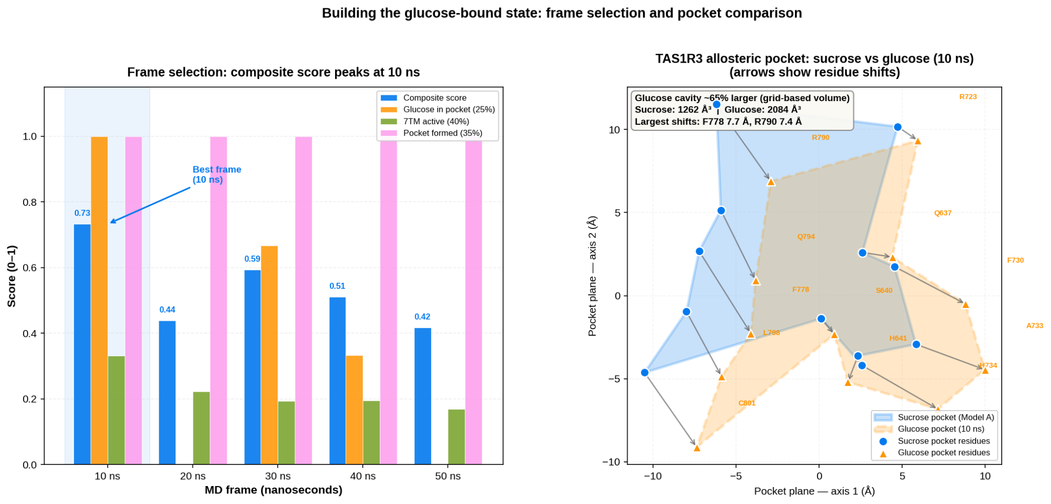
Figure 5. The 10 ns snapshot scores best across all criteria (left); the resulting glucose pocket is genuinely different from the sucrose pocket (right).
The honest part: the simulation was unstable
Reading the frames in time order tells a cautionary story. The glucose oscillates in and out of the pocket — bound at 10 ns, drifting by 20, briefly back at 30, essentially dissociated by 50 ns — and the 7TM slowly over-opens beyond the active state. In other words, the glucose pose isn't stable on this timescale. The 10 ns frame was picked precisely because it captures the receptor before either drift sets in, and a separate check confirmed it's a properly equilibrated state rather than a leftover of the starting structure. But this is a real limitation, not a footnote: the honest read is that the pose needs a better-restrained, shorter simulation (or corrected ligand parameters) before the glucose state can be trusted for fine work. It's a good example of why frame selection has to be sceptical — the average snapshot in this run would have been misleading.
One payoff did survive the scrutiny: the glucose pocket is genuinely different from the sucrose pocket — roughly 2–3 Å shifts in the key side chains and a ~60% larger cavity — which is the whole reason to bother building it separately rather than reusing the sucrose model.
What this workflow really illustrates
The finished model looks authoritative — a clean structure you can rotate on screen. But it's worth being clear about what it is: a composite. The flytrap came from one human experiment. The active 7TM backbone came from a separate, lower-resolution density map. The side-chain identities came from sequence databases. The two missing loops came from an algorithm. The sucrose was chemically edited in. Physics-based minimization glued it all into something self-consistent.
None of that is cutting corners — it's how structural biology routinely bridges the gap between imperfect data and usable models. The discipline is in being explicit about which atoms rest on experiment and which rest on inference, and in validating the result against every independent signature you can find before trusting it. That is the real lesson of this walkthrough: building a structure from a cryo-EM map is less a single act of "solving" it than a sequence of careful, documented decisions — and knowing exactly how much each one can bear.
The cast of structures
| Code | What it provided |
|---|---|
| EMD-70734 | The cryo-EM density map (4.28 Å) of the active "loose" state — source of the active 7TM backbone |
| 9UTB | Full-length human structure (sucralose-bound) — source of the flytrap + linker; its own 7TM was inactive |
| 9UT8 | Apo full-length human structure — used to prove 9UTB's 7TM was inactive |
| 9OQ0 / 9OPX | Inactive 7TM structures — the "off-state" references used to confirm the built 7TM is genuinely a different, active conformation |
| Model A | The built product — full-length, human, active, sucrose-bound |
| Model B | A second built product — glucose-bound active state, selected from a molecular-dynamics run started from Model A |
The active-state structures were reported by Wang et al., Cell Research 2025, and the full-length human structures by Shi et al., Nature 2025.
Map enhancement used CryoSAMU*** (structure-aware multimodal U-Nets for intermediate-resolution maps); automated model building used CryoAtom** (Su et al., Nature Structural & Molecular Biology 2025).*
今すぐVecuraを試す
自分の入力を持って、Vecuraができることを探求しましょう